Fred Senese's post is an excellent starting point. I wanted to add that transforming data in this way is conceptually very useful but distorts parameter estimates because of unequal weighting of data point uncertainty.
The uncertainty of your "zero" data points is probably not negligible. How exactly could you read your gas measurement apparatus? To within 0.1 mL, or 1 mL, or ...? Say it was 0.1 mL, then your "zero" data point in mL is $0 \pm 0.1 \text{ mL}$. And your 70 mL data point is $70 \pm 0.1 \text{ mL}$. When you transform the data by taking the logarithm, however, the uncertainty in your data is unevenly affected. The uncertainty of $\ln \left( 0 \pm 0.1 \text{ mL} \right)$ is approximately $\ln{0.1} - \ln{0}$ which as you are discovering is infinite. The uncertainty in log-space of your 70 mL data point is $\ln{70.1} - \ln{70}$, which is 0.0014. So even though the uncertainty on each data point was the "same" before logarithms, say 0.1 mL, after transformation the uncertainty is as unequal as can be (infinity vs. 0.0014)!
Direct non-linear fitting can fit parameters to data without needing transformations. Here is some R code to do the fitting on your data. Because of the issue related to my comment, I had to include an offset parameter. (An exponential equation tends to a positive value as t approaches zero, not to zero...unless there's an offset.) This method is probably overkill for your particular problem or course, but I wanted to include it in case it's useful to other chem.se readers.
#read the data from the question into R and put it in a data frame
g <- as.numeric(str_split('_0___0___0_____5___10___18____22___28___36___44___51____60____70___', '_{1,5}')[[1]]); g <- g[!is.na(g)]
t <- as.numeric(str_split('0___5___10___15___20___25___30___35___40___45___50___55___60 ____', '___')[[1]]); t <- t[!is.na(t)]

dat <- data.frame(g = g, t = t)

# scale the data to avoid numeric problems taking the exponential of large numbers
dat$g.scaled <- dat$g/max(dat$g)
dat$t.scaled <- dat$t/max(dat$t)

#compare to fitting result by neglecting first three zero points and taking logarithm
dat$ln.g[4:13] <- log(dat$g)
lm(formula = ln.g ~ t, data = dat)

# show data
dat
        g  t   g.scaled   t.scaled
1   0  0 0.00000000 0.00000000
2   0  5 0.00000000 0.08333333
3   0 10 0.00000000 0.16666667
4   5 15 0.07142857 0.25000000
5  10 20 0.14285714 0.33333333
6  18 25 0.25714286 0.41666667
7  22 30 0.31428571 0.50000000
8  28 35 0.40000000 0.58333333
9  36 40 0.51428571 0.66666667
10 44 45 0.62857143 0.75000000
11 51 50 0.72857143 0.83333333
12 60 55 0.85714286 0.91666667
13 70 60 1.00000000 1.00000000

#do direct nonlinear fitting
fit <- nls(g.scaled ~ A0*exp(k*t.scaled)+offset,
           data = dat, start = list(A0 = 1, k = 1, offset = 1))

#do logspace fitting to linear equation by transformation and neglecting first three data points
dat$ln.g[4:13] <- log(dat$g[4:13])
logfit <- lm(ln.g ~ t, data = dat)

#compare predicted values from fit to real data
dat$pred.scaled <- predict(fit)
dat$pred <- dat$pred.scaled * max(g)
dat$logpred[4:13] <- exp(predict(logfit))
require(ggplot2)
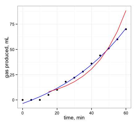
ggplot(data = dat, aes(x = t)) + geom_point(aes(y = g)) + geom_line(aes(y=pred), color = 'blue') + geom_line(aes(y=logpred), color = 'red')

The blue curve is the direct nonlinear fit and the red curve is the linear fit of log-transformed data (dropping the first three data points).
The obtained rate constant is quite different in the two cases! For the direct nonlinear fit, the rate constant is $1.4 \text{ hr}^{-1}$, and for the log-transformed data with linear fit, the rate constant is $0.053 \text{ min}^{-1}$, or $3.2 \text{ hr}^{-1}$!

