Solution to the rate law of first order reaction followed by second order reaction (consecutive)

Question

I'm trying to derive the rate law of a first order followed by second order consecutive reaction:

$$ \frac{\mathrm{d}[\ce{A}]}{\mathrm{d}t}=-k_1[\ce{A}]$$ $$ \frac{\mathrm{d}[\ce{B}]}{\mathrm{d}t}=k_1[\ce{A}]-k_2{[\ce{B}]^2}$$ $$ [\ce{A}](0)=[\ce{A}]_0,\ce{[B]}(0)=0$$

The solution for A is trivial: $$ \ce{[A]}=\ce{[A]}_0\exp(-k_1t)$$

The problem is B, whose rate law ODE is not linear: $$ \frac{\mathrm{d}[\ce{B}]}{\mathrm{d}t}=k_1[\ce{A}]_0\exp(-k_1t)-k_2{[\ce{B}]^2}$$

This is a nonlinear first order ODE, but can be rewritten to a linear second order ODE by substituting $[\ce{B}]$ with: $$[\ce{B}]=\frac{\mathrm{d}y}{\mathrm{d}t}\frac{1}{k_2y}$$

Which gives: $$ -\frac{\mathrm{d}^2y}{\mathrm{d}t^2}+k_1k_2[\ce{A}]_0\exp(-k_1t)y=0$$

The solution is quite complicate and contains Bessel functions of both the first and the second kind:

$$ [B] = \frac{C_1\,{\mathrm{e}}^{-\frac{k_{1}\,t}{2}}\,J_1\left(\frac{2\,{\mathrm{e}}^{-\frac{k_{1}\,t}{2}}\,\sqrt{-\ce{A}_{0}\,k_{1}\,k_{2}}}{k_{1}}\right)\,\sqrt{-A_{0}\,k_{1}\,k_{2}}-\ce{C}_2\,{\mathrm{e}}^{-\frac{k_{1}\,t}{2}}\,Y_1\left(-\frac{2\,{\mathrm{e}}^{-\frac{k_{1}\,t}{2}}\,\sqrt{-A_{0}\,k_{1}\,k_{2}}}{k_{1}}\right)\,\sqrt{-A_{0}\,k_{1}\,k_{2}}}{k_{2}\,\left(C_1\,J_0\left(\frac{2\,{\mathrm{e}}^{-\frac{k_{1}\,t}{2}}\,\sqrt{-A_{0}\,k_{1}\,k_{2}}}{k_{1}}\right)+C_2\,Y_0\left(-\frac{2\,{\mathrm{e}}^{-\frac{k_{1}\,t}{2}}\,\sqrt{-A_{0}\,k_{1}\,k_{2}}}{k_{1}}\right)\right)}$$

There are two arbitrary constants but I only have one condition: $$\ce{[B]}(0)=0$$

So my questions are:

• Is my approach solving the rate law correct ?
• If so, how do I get rid of both constants ?
• Is there any approximated solution to this rate law ?

[update]: The ODE is solved numerically with Runge-Kutta method. The symbolic solution seems correct.

Answer 1

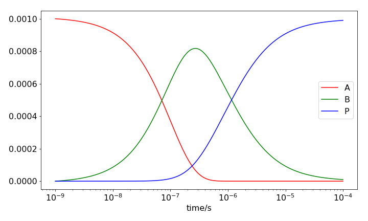
The following code is in Python and uses numpy, scipy and matplotlib that are usually packaged with python. The code will solve the equations $\mathrm{A} \underset{k_3}{\stackrel{k_1}\leftrightharpoons} 2\mathrm{B} \stackrel{k_2} \longrightarrow \mathrm{ P}$ but you can set $k_3$ to zero if you want. (its called km1 in the code). I've used log time spaced points so that a wide time range can be seen. The x axis is log in the plots.

I have used a built in solver, odeint(), buy you could write your own based on the Euler or Runge -Kutta methods.

import numpy as np
import matplotlib.pyplot as plt
from scipy.integrate import odeint

def dX_dt(X, t, const):     # returns rates dEf/dt, only used in odeint()

    k1, km1, k2 = const     # unpack constants needed for calc'n
    A = X[0] 
    B = X[1] 
    dAdt=    -k1*A  +  km1*B*B                 #  rate equations here 
    dBdt=     k1*A  - (km1+k2)*B*B

    f = np.array( [(dAdt), (dBdt)] )           # evaluate equations; 
    return f

C0 = np.zeros(2,dtype=float)
C0[0] = 1.0e-3    # C0= [ A(0), B(0)   ]      # initial concentrations 
numt = 200
t = np.logspace( -9,-4,  numt )    # time as initial power, final power, num points
k1  = 1e7  # 1st order rate const s^(-1)
km1 = 1e6  # 2nd dm^3mol^(-1)s^(-1)
k2  = 1e9  # 2nd  ....
const = [ k1, km1, k2 ]                            # rate constants for calc'n

soln = odeint(dX_dt, C0, t, args = (const,)  )     # solve equations                 
Aval, Bval = soln.T     # extract data

plt.plot(t,Aval,color='red',  label='A')
plt.plot(t,Bval,color='green',label='B')
plt.plot(t,C0[0]-Aval-Bval,color='blue',label='P')
plt.xscale('log')
plt.legend()

plt.tight_layout()
plt.show()

The figure shows the populations vs (log) time