How to determine uncompensated or solution resistance of a 3 electrode setup for IR correction?

Question

To correct for ohmic losses from the potential drop across the electrolyte due to the distance between the electrodes, electrochemical impedance spectroscopy (EIS) is typically employed to measure this electrolyte resistance (R_s).

Currently I think that the Nyquist plot (where each point has a frequency and a real and imaginary impedance) needs to be fitted to an equivalent Randles circuit, which then allows determination of the R_s. The one in particular should be

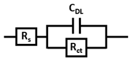
What I'm hoping to achieve is something like this, as well as to finding the solution resistance to calculate iR drop:

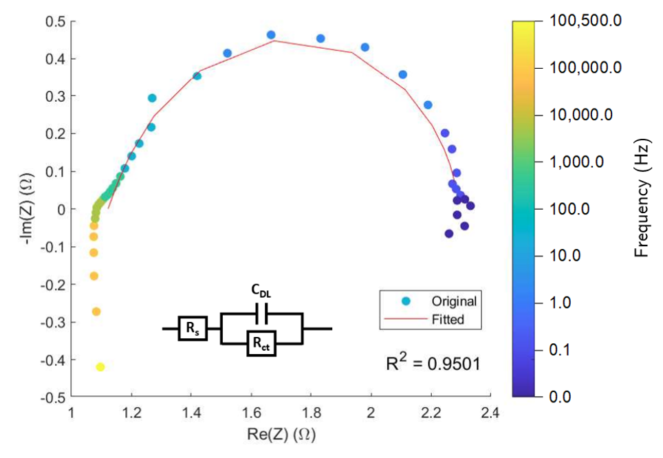
How could this be done? Here is an example of the data I have:

freq in Hz	Re(Z) in Ohm	-Im(Z) in Ohm
1.0000371E+005	1.2838266E+000	-4.7236100E-001
6.7491828E+004	1.2575362E+000	-2.9951397E-001
4.5557453E+004	1.2489935E+000	-1.9674678E-001
3.0748963E+004	1.2461497E+000	-1.3021792E-001
2.0756010E+004	1.2463084E+000	-8.5121296E-002
1.4010540E+004	1.2458339E+000	-5.3675517E-002
9.4523906E+003	1.2463924E+000	-3.2538280E-002
6.3779312E+003	1.2452079E+000	-2.0627080E-002
4.3063779E+003	1.2464187E+000	-7.8994250E-003
2.9059297E+003	1.2512513E+000	-7.8682322E-004
1.9631409E+003	1.2515490E+000	5.4816552E-003
1.3237295E+003	1.2460785E+000	5.2928450E-003
8.9414160E+002	1.2562760E+000	1.8789139E-002
6.0287787E+002	1.2608212E+000	2.7019683E-002
4.0721527E+002	1.2652799E+000	3.7225980E-002
2.7473624E+002	1.2735685E+000	4.8571289E-002
1.8553433E+002	1.2811457E+000	6.3650906E-002
1.2520035E+002	1.2927077E+000	8.0610186E-002
8.4486298E+001	1.3058180E+000	9.9876016E-002
5.7063412E+001	1.3209573E+000	1.3237002E-001
3.8485222E+001	1.3433586E+000	1.6853021E-001
2.5972410E+001	1.3701465E+000	2.2286178E-001
1.7516815E+001	1.4067172E+000	2.9568654E-001
1.1837119E+001	1.4666675E+000	3.9322603E-001
7.9882402E+000	1.5431337E+000	5.2406406E-001
5.3879313E+000	1.6745517E+000	6.8878186E-001
3.6371040E+000	1.8626976E+000	8.5898042E-001
2.4567609E+000	2.1712506E+000	1.0030348E+000
1.6587046E+000	2.5552261E+000	1.0842789E+000
1.1199110E+000	2.9400694E+000	1.0472580E+000
7.5526887E-001	3.2742524E+000	8.9296573E-001
5.0942224E-001	3.5140378E+000	7.0039696E-001
3.4379947E-001	3.6070650E+000	5.1860118E-001
2.3239036E-001	3.6902442E+000	3.5689598E-001
1.5689009E-001	3.7351005E+000	2.2994351E-001
1.0589487E-001	3.7651119E+000	1.3973090E-001
7.1417451E-002	3.7816873E+000	3.9920006E-002
4.8211023E-002	3.7677062E+000	-8.1531301E-002
3.2556150E-002	3.7300577E+000	-1.7607281E-001
2.1934874E-002	3.6879458E+000	-1.6583309E-001
1.4821894E-002	3.6872365E+000	-1.9536464E-001
1.0009173E-002	3.6411600E+000	-1.3885058E-001

Answer 1

I have reluctantly appended some code written in Python as a Jupyter notebook ( Jupyter notebooks was used via Anaconda and is free to use), reluctantly because the code not v. elegant but should be usable to start with, after a little effort. The code should also run using Visual Studio Code, which is also free to use.

The function to fit is in 'Model'. I used $R_s+R_c/(1+iR_cC\omega)$ and as you can see the fit is poor suggesting that the data fits a more complicated model. You should be able to change the equation used to a more suitable form.

There is computed test data. Towards the bottom of the code there is a True or False switch to change between reading real data and using test data. The real data file should be comma separated in three columns in the order in your post and have no header or other characters etc. You will need to generate your own data file and change the name in this code if needs be. This file should be in the same folder as the code.

# import all python add-ons etc that will be needed later on. Python 3 is used
# the follwing line is only used in Jupyter notebooks
%matplotlib inline    

import numpy as np                      # import fast numerical library
import matplotlib.pyplot as plt         # import plotting library
from scipy.optimize import leastsq      # import non-lin least squares routine 
plt.rcParams.update({'font.size': 14})  # set font size for plots

def read_data():
    filename ='nyquist-data.txt'  #  The numbers are in 3 columns comma separated, freq, real, imag 
                                  #  No other text and no comma at end of lines 
    w = []
    rdata = []                    # real floats
    idata = []                    # imag floats
    with open(filename) as f:
        for line in f.readlines():
            f_list = [ float(i) for i in line.split(",") ] # separate out numbers comma separated
            w.append(f_list[0])
            rdata.append(f_list[1])
            idata.append(-f_list[2])
    w = np.array(w)                            # make w into array
    data = np.zeros(len(w),dtype = complex)    # make new array of complex numbers
    data.real = rdata
    data.imag = idata
    
    a = 5                               # used to limit range of experimental data use [:] for all data
    b = 38
    return w[a:b], data[a:b]            # return data but leave out messy bits either end

#----------------------------    
def make_data(Rs,Rc,C):                  #  For testing only. Noise added 
    n = 10000                            #  number of data points
    w = np.linspace(0.0,n,n)             # range of frequency, 0 to n, and n points
    rng = np.random.default_rng()
    z = model(w,Rs,Rc,C) + 0.01*(rng.random(n) + 1j*rng.random(n))  # 1j is sqrt(-1)
    return w,z
#-----------------------------

def model(w,Rs,Rc,C):                    # Change equation here as necessary
    Z = Rs + Rc/(1.0 + Rc*C*1j*w )       # 1j is sqrt(-1) 
    return Z                             # z is complex array, i.e has real and imag parts
#----------------------------

def resids(params,w,z):
    Rs, Rc, C = params
    diff =  model(w, Rs, Rc, C) - z      # calculates residuals using current set of parameters 
    zri = []                             # make new  1D array as real part, imag part, real, imag... etc
    for a, b in zip(diff.real,diff.imag):
        zri.append(a)
        zri.append(b)
    return zri                           # we can only input 1d array to least squares, i.e. not complex array
#----------------------------

def do_calc(params):
    vals = leastsq(resids, params, (w,z) )  # w, z is the data, resids is routine to calc resduals
    Rs = vals[0][0]                         # get fitted parameters from vals 
    Rc = vals[0][1]
    C  = vals[0][2]
    sum_resids = sum( abs(model(w, Rs, Rc, C) - z)**2 )
    print('{:s} {:6.3f} {:6.3f} {:6.3f} {:s} {:6.3f}'.format('values Rs, Rc, C are',Rs, Rc, C ,'sum^2 resids', sum_resids) )
    return Rs,Rc,C
#-----------------------------

test_calc = False # True to use test data   # False to read in your data
if test_calc == True :
    Rs, Rc, C = 2.5, 1.5, 0.01   # used to make test data 
    w, z = make_data(Rs,Rc,C)    # w is frequency, z complex array real & imag values
else:
    w, z = read_data()

params = [0.5, 2.0, 0.01]        # Rs, Rc, C initial values or fitting

fitRs, fitRc, fitC = do_calc(params)

zre = model(w,fitRs,fitRc,fitC).real  # make data from fitted params to plot on Nyquist plot
zim = model(w,fitRs,fitRc,fitC).imag

plt.plot(zre, -zim, color='red',linewidth=5,alpha=0.3)  # wide red-ish line

plt.scatter( z.real, -z.imag ,s = 5, color='blue'  )    # data points 
plt.ylabel('-Z(im)')
plt.xlabel('Z(re)')
plt.tight_layout()
plt.show()

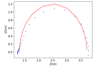
The fit to the data is shown below, the params are Rs, Rc, C are $1.311, 2.408, 0.238\; \sum^2\;= 0.232$. The fit is the thick red line, the data points are blue dots. The fit is made to ignore the first few and last few data points but is still a poor fit to the data. The results are not particularly sensitive to the initial guesses.