1
$\begingroup$

An article on Khan-Academy, states the following:

The overall reaction rate is determined by the rates of the steps up to (and including) the rate-determining step

Here, it says that rate is determined by steps before and including that of RDS. But from what I know the rate is determined by one single elementary reaction, which is the slowest, that is, the RDS. So why does it include steps previous to RDS?

(I would appreciate an example of this)

$\endgroup$
4

2 Answers 2

3
$\begingroup$

The interpretation of the statement depends on exactly what is meant by "overall rate."

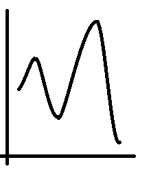
reaction coordinate

The rate-determining step corresponds to the largest free energy difference from a transition state to any preceding stable state (reactant or intermediate).

In the example above, the biggest forward barrier is from the reactant to the second transition state, so the second step is rate-determining. However, the barrier, as identified above, is comprised of both the first and second step, so they both figure into the overall rate of the reaction, as determined by the slow step.

EDIT:

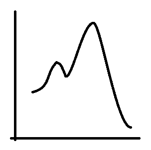
Based on comments, I think a clarification is in order. Note that the above conclusion is not true in the general case. You could make the indicated claim for the depicted reaction specifically, but not, for example, in the case below:

reaction coordinate 2

The second step here is still rate-determining because the transition state is involved in the largest barrier. However, the biggest barrier is from the intermediate to the second transition state. In this example, I would not say that the overall rate depends on the first step.

$\endgroup$
6
  • $\begingroup$ "they both figure into the overall rate of the reaction" - do they? How? $\endgroup$ Commented Aug 4, 2020 at 8:40
  • $\begingroup$ They must because the rate-determining step has a corresponding $\Delta G^{‡}$ that spans the reactant and the second transition state. The barrier is made up of both the first and second step. In this example, if you were to write the rate law, it would have to include the rate of the first step, but rate constant for step 1 will be absorbed into the overall rate constant, via the equilibrium from the reactant and the first intermediate. @user6376297 $\endgroup$
    – Zhe
    Commented Aug 4, 2020 at 15:46
  • $\begingroup$ I see. Yes, OK, if you consider equilibrium constants as ratios of rate constants then they 'figure' in the overall rate constant. But I think this confuses the point. The OP, with whom I agree, was puzzled by a statement seeming to indicate that the rate (constant) of the overall reaction is influenced by the rate (constants) of the RDS and of the steps that precede it. Instead, under the RDS approximation the preceding steps can only influence the overall rate constant by their thermodynamics, not by their kinetics. It does not matter how fast they are, just that they are 'much faster'. $\endgroup$ Commented Aug 4, 2020 at 18:25
  • $\begingroup$ To be more explicit. In the example I posted below, the equation for $C(t)$ when the first step is fast and the second step is the RDS only contains rate constant $k_B$, not $k_A$. The numerical value of $k_A$ has no bearing at all on it. Even if the first step were a fast reversible reaction, it would still only influence the overall $C(t)$ by its equilibrium constant, indeed as you say. It will not be necessary to know the rate constants of the direct and inverse reactions. This IMO is no minor difference, and it does make a big difference (operationally) when one models such systems. $\endgroup$ Commented Aug 4, 2020 at 18:31
  • $\begingroup$ @user6376297 It's not so much that the rate constant matters. It's that the first step matters. The overall rate includes contributions from both steps, and therefore, you cannot ignore the first step. Is the rate constant explicit? No, it is not. But if you remove the first step, you've changed the kinetic properties of the system. $\endgroup$
    – Zhe
    Commented Aug 4, 2020 at 19:58
1
$\begingroup$

It is perhaps worth noting that the 'rate determining step' is an approximation.

It is technically possible to model any reacting system without it, by using numerical methods.
It is even possible to model certain systems fully analytically.

Take for instance a sequence of 2 consecutive irreversible reactions:

$\ce{A ->[k_A] B ->[k_B] C}$

which is described by:

$\frac{dA}{dt}=-k_A A$
$\frac{dB}{dt}=+k_A A-k_B B$
$\frac{dC}{dt}=+k_B B$

This system of differential equations has an analytical solution. Assuming that only $\ce A$ is present at $t=0$, at a concentration $\ce{A(0)}$:

$A(t) = A(0) e^{-k_A t}$
$B(t) = \frac {k_A A(0)}{k_B-k_A} [e^{-k_A t}-e^{-k_B t}]$
$C(t) = \frac {A(0)}{k_B-k_A} [k_B (1-e^{-k_A t}) -k_A (1-e^{-k_B t})]$

Suppose that the first reaction is 100 times faster than the second ($k_A = 1, k_B = 0.01$).
If you plot the 3 concentrations for $t \in [0,100]$, you will see $A$ disappear quite fast and $B$ reach its maximum when $C$ is still quite low.
In other words, you can assume that the second step is the 'rate determining' one, i.e. assume that all $A$ almost immediately turns into $B$, so $B(0) \approx A(0)$, and model only the second and third reaction:

$B(t) \approx A(0) e^{-k_B t}$
$C(t) \approx A(0) [1-e^{-k_B t}]$

The same result can be reached directly from the exact analytical solution, by setting $k_A >> k_B$:

$B(t) \approx \frac {k_A A(0)}{-k_A} [-e^{-k_B t}] = A(0) e^{-k_B t}$
$C(t) = \frac {A(0)}{k_B-k_A} [k_B (1-e^{-k_A t}) -k_A (1-e^{-k_B t})] \approx \frac {A(0)}{-k_A} [-k_A (1-e^{-k_B t})] = A(0) [1-e^{-k_B t}]$

Suppose instead that the first reaction is 100 times slower than the second ($k_A = 0.01, k_B = 1$), and plot the 3 concentrations for $t \in [0,1000]$.
You will see $A$ disappear according to a rather typical first order decay, $C$ form equally typically, whereas $B$ remains barely visible at the bottom of the plot (in some contexts $B$ would be called a 'stationary intermediate').
You can assume that the first step is the 'rate determining' one, i.e. assume that $\frac {dB}{dt} \approx 0$, and consequently $\frac {dC}{dt} = k_B B \approx k_A A$, and model only the first and third reaction:

$A(t) = A(0) e^{-k_A t}$
$C(t) \approx A(0) [1-e^{-k_A t}]$

Here, too, the same result can be reached directly from the exact analytical solution, by setting this time $k_A << k_B$:

$A(t) = A(0) e^{-k_A t}$
$C(t) = \frac {A(0)}{k_B-k_A} [k_B (1-e^{-k_A t}) -k_A (1-e^{-k_B t})] \approx \frac {A(0)}{k_B} [k_B (1-e^{-k_A t})] = A(0) [1-e^{-k_A t}]$

In both these 'extreme' cases, the approximate curves described by the 'rate determining step' approximation fit quite closely the exact curves, but there is nothing better than the latter, for a more accurate account of the system.
Also considering that one does not know a priori if a given approximation holds true or not for a particular system.

It is sufficient to set $k_A = 1, k_B = 1.01$, i.e. have two consecutive reactions of comparable rate, and plot the exact concentrations for $t \in [0,10]$, to see that $C(t)$ is not really well described by either approximate rds solution.

Luckily these days there are plenty of excellent software solutions allowing to model systems of any complexity via very accurate numerical methods.

$\endgroup$
1
  • $\begingroup$ It might be worth mentioning that the RDS approximation may break down completely in catalytic cycles (or yields the right observation by accident). $\endgroup$ Commented Aug 4, 2020 at 7:23

Your Answer

By clicking “Post Your Answer”, you agree to our terms of service and acknowledge you have read our privacy policy.

Not the answer you're looking for? Browse other questions tagged or ask your own question.